ML System Design — Language Translation

Design a ML System to translate post or comments on a news feed such as Facebook/LinkedIn.
Type of ML Problem
There are 2 problems here:
- Detect the language of the post/comment made by author
- Translate the post/comment into viewer’s language
We will assume that for the 1st problem we already have a language classification model. This could be a multi-class softmax classifier where the output is a probability distribution over all possible languages.
Our main focus is the 2nd problem here.
This is a sequence to sequence supervised learning problem i.e. given a sentence with sequence of words in one given language (authors language), translate the sentence into another language (viewers language).
We can use sequence-to-sequence learning with either LSTM based or Transformer based encoder-decoder networks.
What are the features ?
The raw features for the model are the words from the source and target language.
For e.g. if the source language is English and target is Hindi:
source: “How are you ?”
target: “Aap kaise hai ?”
Then the words are “How”, “are”, “you” from source and “Aap”, “kaise”, “hai” from the target.
In order to handle spelling errors and missing characters in production, instead of whole words we can use character n-grams. For e.g. with 2-character n-grams, we will have the following features:
source: ["Ho", "ow", "w ", " a", "ar", "re", ...]
target: ["Aa", "ap", "p ", " k", "ka", "ai", ...]
For k-character n-grams, we have a sliding window of size k over the source and target sentence with a step size of 1. Instead of using a single k, we can also use a range of k such as k=1 to 3. For e.g. if the actual word is “How” and it is mistakenly typed as “H0w”, with k=2 we would have [“H0”, “0w”] both of which are out of vocabulary (OOV). But with k=1 to 2, we would have [“H”, “0”, “w”, “H0”, “0w”], we have 2 out of 5 features (“H” and “w”) that should also have been part of the correct word.
Other features we can use are (but may not be required if we use neural networks to learn more complex features):
- POS and NER tags
- isNumeric, isTitle, isAlphanumeric etc.
How to get training and testing data, how to get labels ?
To develop the translation model, we would need sentence pairs for each pair of languages.
Assuming that our system can work with 50 different languages, thus we should have 50*50=2500 different models corresponding to each language pair. Some strategies for obtaining training data are as follows:
- Explicit labelling — Manually create sentence pairs using language experts. But it would take a long time to create enough training data.
- Use a single anchor language — For e.g. using only English language, generate translations for the remaining 49 languages using Google Translate or some other existing service.
We can create CSV files with 50 columns each corresponding to a language with the first column containing the sentence with the anchor language.
For each model M(a, b) where a is the source language and b is the target language, we can extract from each row, sentences from the 2 columns corresponding to languages a and b:
df = pandas.read_csv('data.csv')
df_a_b = df[['language_a', 'language_b']]where df is the Pandas dataframe corresponding to the CSV file training dataset.
This assumes transitive property in languages i.e. if A->translates to->B and A->translates to->C then B->translates to->C which may not hold true in specific scenarios.
How to select the sentences for the anchor language ?
- Select sentences of different lengths.
If we select only long sentences, then the model may not learn the “meaning” of short phrases properly which is essential to translate longer sentences. Similarly if we only select short sentences then system may only learn to form “incomplete” target sentences when we input long source sentences. - From different domains such as science, politics, news, sports etc. so that model is not biased towards words/phrases from particular domains.
- Using sentences from historical posts/comments so that data is from similar domains. For e.g. sentences in posts/comments in a social network are more informal and may contain memes, sarcasms, abbreviations etc. which would be greatly different if we only use Wikipedia articles instead.
- Introducing random spelling errors in sentences or randomly removing words from between sentences to simulate production scenarios.
What options are there instead of training O(N²) models for N languages ?
One option is to train 2N models but in a binary tree format.
With the anchor language A as the root, train 2 models with it as the source and targets as B and C and 2 models with A as target and source as B and C. Similarly for each B and C train 2 models as source and 2 models as targets and so on.
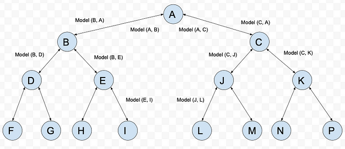
To translate language X to Y, one way is to do Depth First Search from X till we find Y. At each step, we call a translation model to translate P to Q along the path. Number of models invoked is O(N).
Another approach is using Binary Uplifting + Lowest Common Ancestor.
Compute the ancestors of each node (1, 2, 4, 8,…) using Binary Uplifting strategy. Space complexity is O(N*loglogN). Because maximum depth from root to any leaf node is O(logN).
To translate language X to Y, first we find the Lowest Common Ancestor Z of X and Y, then translate X to Z in O(logN) model invocations and then translate Z to Y in another O(logN) model invocations. In the worst case we have to traverse diameter of the tree i.e. O(2*logN).
This again assumes that languages are transitive i.e.
A->B, B->C implies A->C.The tradeoff here is that although we are training O(N) models instead of O(N²) but at inference time we need to evaluate O(logN) models instead of O(1) models.
What feature pre-processing steps are required ?
- Remove outliers — Single word sentences with very rarely occurring (frequency is 1) words can be removed. Similarly sentences with more than 50% of the words not in vocabulary can also be removed from training dataset.
- Replace non-UTF8 and special characters with blank spaces.
- Marking [start] and [end] — For each target sentence add a [start] word at the beginning and a [end] word at the end. This will be used to signal when to start and stop generating further words in the target language.
- Replace punctuations — Punctuations in the target language are replaced with special words. For e.g. “?” will be replaced by [?] and so on.
- Lowercasing of words.
How to compute the feature representations ?
To train the LSTM or the Transformer models, we need to vectorize the word and character n-gram features:
- Sort all the character n-grams (k-character n-grams from above) and store them in a list.
- In the given sentence, convert each k-character n-gram into its corresponding index in the sorted list from above. Use index+1 instead of index because we want to start calculations from 1.
"How are you" -> ["ho", "ow", "w ", " a", "ar", "re", ...] -> [67, 150, 239, 13, 100, ...]Since training of LSTM or Transformer networks require that all sentences in a single batch have the same length, thus assuming that the maximum length of any sentence is N, all sentences smaller than N will be padded at the end with 0’s (since we are starting our feature values from 1 onwards above).
[67, 150, 239, 13, 100, 45, 0, 0, 0, 0, 0....0]After this, each sentence vector of length N is then transformed into a one-hot encoding 2D matrix of dimensions N*V where V is the vocabulary size.
[[0,0,...0,1,0,0,...0],
 [0,0,0,....0,0,1,..0],
...]
Where to store the feature representations ?
We need to store the sorted list of n-grams in the vocabulary for all languages as well as an inverted index (HashMap) from the n-gram to the index. Both of these can be stored in Redis. For persistence we can also store them in Cassandra.
Table: vocabulary in Cassandra
(word_id, word, language, index)In Redis:
HashMap A: (word, language) -> indexHashMap B: (language, index) -> word
During training of the model, we would also be computing the embeddings for the words using an embedding layer. Each embedding corresponding to a feature will be stored in Redis HashMap for real time inferencing:
HashMap (key:feature_id) -> [embedding]Since we will be training the models using Transformer networks, in order to maintain the positional information associated with each word (as in RNN or LSTM), we will use Positional Embeddings apart from word embeddings.
pos_embed(i, 2j) = sin(i/10000^(2j/d))
pos_embed(i, 2j+1) = cos(i/10000^(2j/d))
i.e. for an embedding of length d, for the i-th feature, at every odd index (2j+1) compute the cosine and at every even index compute the sine value.
The final embedding is the summation of word embedding and pos_embed.
Since the positional embeddings are independent of the actual word, we can cache these values so that we do not have to do expensive sine and cosine calculations at inference time.
How to train the model using the features ?
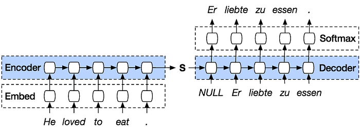
Approach 1: Using LSTM Seq-To-Seq Encoder-Decoder
Training Phase:
- Each n-gram for the source language is converted into an integer index and then one-hot encoding before passing to the embedding layer.
- The embedding layer before the encoder is used to convert the one hot encoding of the n-grams into dense vector.
- The dense vector from the embedding layer is passed to the encoder LSTM. Each unit of LSTM computes an internal cell state ‘c’ and a hidden state ‘h’ which are passed to the next unit.
- The hidden state ‘h’ from the last unit of encoder is used as input state for the decoder network.
- The target of the decoder is left shifted by one position from the input for the decoder. i.e. if the input is [[start], “aap”, “kaise”, “hai”, [end]], then the corresponding target is [“aap”, “kaise”, “hai”, [end]]. Thus [start] as input is used to predict “aap”, “aap” as input is used to predict “kaise” and so on.
- Each LSTM unit of decoder produces an output apart from the states ‘c’ and ‘h’. ‘c’ and ‘h’ are passed to the next cell unit and the output is passed through a dense layer and then a softmax layer which emits probabilities for each word at position t.
- Each unit is then trained using categorical cross-entropy loss function with the actual target word at position t.
Inference Step:
- Similar to the training, the encoder network produces the states ‘c’ and ‘h’ using the source language as input. These states are used as input states for decoder network.
- During inferencing we do not have the true translation as input as in the training phase.
- Predict the word with the highest probability at position t. Use this word as input along with the states ‘c’ and ‘h’ from the current unit as inputs to the next cell unit.
- Repeat this until we encounter [end] or maximum length of target sentence.
Approach 2: Using Transformer Network with Multi-Headed Attention
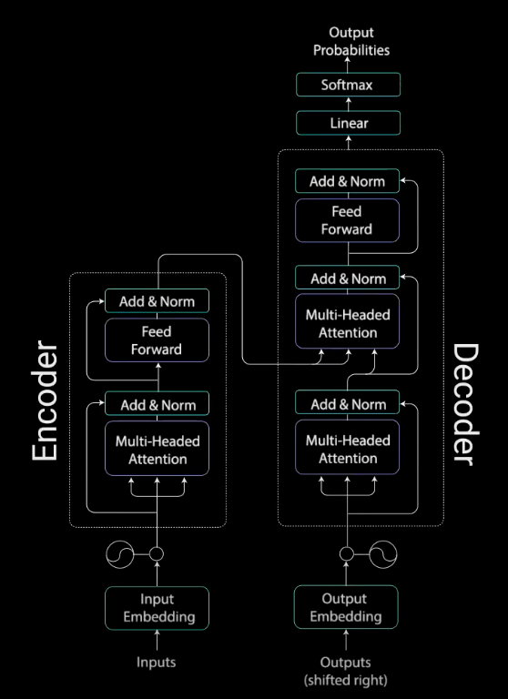
Instead of using LSTM, we use attention to determine how important an n-gram is relative to all other n-grams.
- Although LSTM handles vanishing gradient problem better than RNN but still it cannot handle very long range dependencies when input and output sentences are very long.
- LSTM is sequential in nature and thus cannot be parallelized. In attention networks we can parallelize the weight calculations for each unit.
Following are the steps to train the model:
- Split the dataset into training, testing and validation (usually 80–20)
- Do the hyper-parameter tuning (number of heads, embedding dimension, number of stacks, dropout etc.) using grid search cross validation (K-fold).
- The best hyper-parameters are chosen based on the BLEU score on validation dataset averaged over all the K runs.
- Final model is trained on the entire training data with the best hyperparameters.
How to evaluate the model offline ? Metrics ?
BLEU Score
How to save the model and model weights, architecture etc. ?
Tensorflow models can be saved in multiple different ways.
- During training i.e. after each epoch we can save the model checkpoints using callbacks (so that even if we stop training we can start from wherever we have left). The model checkpoints consists of the model weights and index files. If the network is sharded, then weights corresponding to each shard are stored in separate files and the index file is like an hashmap from the weight (source layer, source node, dest layer, dest node) to the shard.
- After training, the model can be saved in SavedModel format which stores the model as Protobuf file.
- All of these checkpoints and protobuf files can be uploaded to S3 after training is completed.
<bucket_name>/<date>/<version>
How to deploy the inferencing codes into production ?
- Instead of explicitly loading the Tensorflow SavedModel file and other index files for inferencing within Flask, we can use TF Serving to do that for us.
- But TF Serving do not handle feature preprocessing. For that we need Flask.
- Create Flask endpoints for inferencing.
- To make Flask multithreaded, use Gunicorn on top of Flask.
- Use Github+Jenkins to build a CI/CD Pipeline.
- Whenever a PR for the inferencing codes is created in Github, trigger Jenkins build i.e. run any unit and integration test cases and if all test cases passes, then build docker image and deploy the docker image in a Kubernetes cluster.
- Instead of a single docker container running both TF Serving and Flask+Gunicorn, create 2 separate docker containers so that they are decoupled.
- In Kubernetes, we would have 2 deployments and 2 services coresponding to the TF Serving and Flask/Gunicorn server.
- Use at-least 3 replicas for the pods running the docker services to allow for load balancing.
How to monitor the models in production ?
Setup logging and observability with Datadog or Cloudwatch (if using AWS).
Some performance metrics we can track are:
- Number of 5xx errors in the last 5 minutes.
- P99 latency every 5 minutes.
- Number of requests per second.
- CPU load across different nodes running the inferencing service.
- Memory usage across different nodes running the inferencing service.
- Number of Exceptions in the last 5 minutes.
Model metrics we should track:
- Data drift — For each feature pre-compute the mean and variance in the training dataset. In production compute the mean and variance of feature values in streaming way and after every 5 minutes, compute the KL Divergence between the training and production values.
How to do online evaluation ?
One metric we can use is how many engagements are made for each post after some user clicks on “Translate” button. Engagements here means Like, Comment, Share, Send Friend Request, Follow Request etc.
Create a table for tracking user activities on posts, for e.g.:
(post_id, user_id, activity, timestamp)
Then select count of all activities after activity=’CLICK_TRANSLATE’ based on timestamp and user_id.
SELECT post_id, COUNT(activity) as num_activities FROM(SELECT * FROM activities a
INNER JOIN
(SELECT user_id, MIN(timestamp) FROM activities WHERE activity="CLICK_TRANSLATE" GROUP BY user_id) b
ON a.user_id=b.user_id AND a.timestamp > b.timestamp AND a.timestamp >= NOW()-'30 days')GROUP BY post_id
Each post is randomly assigned to either an existing model running in production (model 0) or the new model we want to deploy (model 1). Translations are served from either model 0 or model 1.
For each post in model 0, obtain the engagement counts from the above query, similarly for all posts from model 1. Then using KS Test, test how significant is the improvement in the engagement with model 1 vs. model 0. We can use engagement data from the last 30 days.
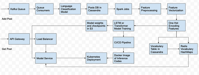
Pipeline
References
- https://keras.io/examples/nlp/neural_machine_translation_with_transformer/
- https://towardsdatascience.com/illustrated-guide-to-transformers-step-by-step-explanation-f74876522bc0
- https://jalammar.github.io/illustrated-transformer/
- https://cloud.google.com/translate/automl/docs/evaluate
- https://aclanthology.org/P02-1040.pdf
- https://blog.keras.io/a-ten-minute-introduction-to-sequence-to-sequence-learning-in-keras.html