ML System Design — Surge Price Prediction

Design a ML system to predict surge multiplier for a trip for Uber/Lyft. Surge multipliers are limited to the set of [1.0, 1.25, 1.5, 1.75, 2.0, 2.25, 2.5]
Type of ML Problem
Note that if we solve it as a multiclass classification problem (where the classes are surge multipliers), then the loss function (cross-entropy or hinge loss) penalizes a prediction of 1.0 for a true label of 2.5 same as it would penalize a prediction of 2.25 but 2.25 is actually more reasonable than 1.0 when the actual should be 2.5.
If we solve it as linear regression problem, then prediction could be any real number. It is upto us then to map a prediction to one of the classes above.
One possible approach is to use Ordinal Regression/Classification.
What are the features ?
We can use some of the following set of features for our model:
- Estimated distance of trip.
- Estimated duration to complete the trip.
- Estimated wait time for cab to arrive at pickup point.
- Pickup location (Quad Tree grid id)
- Drop location (Quad Tree grid id)
- Number of available cabs within a radius of 5KM. (Supply)
- Number of cabs with drop location within a radius of 5KM. (Supply)
- Number of pickup requests in the queue within a radius of 5KM (Demand)
- Hour of the day
- Day of the week
- Number of bookings made by user in last 30 days.
- Number of bookings with surge multiplier X in last 30 days.
- Number of bookings made by user for same (pickup, drop) location pair in last 30 days.
- Type of pickup location (office, pub, sports arena, temple, etc.)
- Weather data — Is it raining, Temperature, Humidity, Wind Speed
… and so on.
How to get training and testing data, how to get labels ?
Store the completed trips data into a big data databases such as Hadoop or Hive with following trip metadata:
(ride_id, user_id, driver_id, quad_tree_src_grid, quad_tree_dst_grid, city, country, distance, ride_duration, ride_type, wait_time, hour_of_the_day, day_of_week, booking_time, surge_multiplier)
Since it is not really a good idea to identify the trips by latitude and longitude, we can group nearby pickup and drop locations in the map using Quad Tree.

Since it is infeasible to track the number of available cabs within 5KM for every trip we can independently track these data using Count Min Sketches.
Create multiple count min-sketches corresponding to different time intervals. Lets say one sketch corresponds to a 10 minute interval. In the next interval a new sketch is created.
Each sketch has D independent hash functions and width of each hash function is W.
Whenever an event from driver’s GPS arrives along with latitude and longitude, convert the lat and long to a quad tree grid id, compute Hash_i(1toD)(grid id) % W and increment the value of those D cells by 1.
Similarly for the other feature: Number of pickup requests in the queue.
For number of bookings made by user we can run Spark SQL jobs to run aggregate queries on the Hive database.
SELECT user_id, COUNT(*) as count FROM trips WHERE booking_time <= NOW()-'30days' GROUP BY user_idSELECT user_id, surge_multiplier, COUNT(*) as count FROM trips WHERE booking_time <= NOW()-'30days' GROUP BY user_id, surge_multiplierSELECT user_id, quad_tree_src_grid, quad_tree_dst_grid, COUNT(*) as count FROM trips WHERE booking_time <= NOW()-'30days' GROUP BY user_id, quad_tree_src_grid, quad_tree_dst_grid
Since we want to train an ordinal regression model, instead of using the surge_multipliers as class labels (multiclass classification) or real numbers (linear regression), we can encode the multipliers as follows:
- 1.0 — [1,0,0,0,0,0,0]
- 1.25 — [1,1,0,0,0,0,0]
- 1.5 — [1,1,1,0,0,0,0]
- 1.75 — [1,1,1,1,0,0,0]
- 2.0 — [1,1,1,1,1,0,0]
- 2.25 — [1,1,1,1,1,1,0]
- 2.5 — [1,1,1,1,1,1,1]
Now if we train a Neural Network with 7 output nodes (each output node applies a sigmoid activation to its input) and use categorical cross entropy loss function:
L = sum_j(1 to 7) -true_j*log(pred_j)Then the loss when the true is 2.5 — [1,1,1,1,1,1,1] and pred is 1.0 — [1,0,0,0,0,0,0] is greater than when pred is 2.25 — [1,1,1,1,1,1,0] because we are adding up the loss term from each output node.
During prediction we map each sigmoid output node to 0 if pred_j < 0.5 else 1.
What feature pre-processing steps are required ?
- Handling correlated and less important features
- Use PCA to merge correlated features.
- Select important features to train by using random forest or gradient boosted trees feature_importance output. - Handling missing values and NaNs
- Replace with mean or median in case of numerical values
- Replace with mode in case of categorical value.
- Remove trips where surge_multiplier is missing. - Outlier detection
- Remove trips where there were extreme weather conditions such as cyclone etc.
- Remove trips for some special occasions such as political processions or huge trafic jams etc.
- We can omit trips where time taken or distance lies outside mean + 2*sd value among all trips. - Feature scaling
- Distance, time, number of cabs etc. all have diferent scales.
- We can normalize the each feature value between 0 and 1 by doing (x-min(x))/(max(x)-min(x)) where x is the feature value and min(x) is the minimum value of the feature across trips.
How to handle class imbalance ?
Number of trips with surge_multiplier=1 will be far higher than number of trips with other surge_multipliers.
Possible solutions are:
- Using SMOTE, generate synthetic data points for the minority classes.
- Let C be a minority class (surge_multiplier=2.25)
- Select K random pairs with replacement from class C.
- For each pair of points Pi and Pj, generate a new point Pk = Pi + r*Pj where 0 ≤ r ≤ 1 is a random number between 0 and 1. - Downsample trips with surge_multiplier=1 i.e. select K random trips with surge_multiplier=1 where K is minimum number of trips among all classes.
- Train multiple models with random sampling and take average of all model prediction. For each model sample equal number of trips from each class.
How to compute the feature representations ? Handle high cardinality features ?
For numerical features (distance, duration, wait time, number of cabs etc.) we can keep the values as it is (after doing feature scaling) or we can do quantile bucketing.
In quantile bucketing the buckets are not fixed size but the number of trips in a bucket are fixed. For e.g. with distance feature, sort the distances first.
D1 ≤ D2 ≤ D3 …. ≤ Dn
Then if the bucket size is K, the first K i.e. D1 to Dk goes into bucket 1, then Dk+1 to D2k goes into bucket 2 and so on. Thus instead of n feature values we have n/K feature values:
D’1, D’2 , … D’n/K
where D’1 = (D1+…+Dk)/K and so on.
For categorical features (such as pickup/drop location, hour, day of week, type of location, weather condition etc.), we can do one hot encoding.
Since number of pickup/drop locations could be in millions, the vectors could be really sparse.
One strategy is to do bucketing. Compute the frequency of trips per location.
Let the location and frequencies of trips sorted in descending order be:
(L1, F1) (L2, F2) … (Ln, Fn) where F1 ≥ F2 ≥ …
Then starting from the 1st location add up the frequencies until the ratio of (F1+F2+…+Fk)/(F1+F2+…+Fn) ≥ 0.9 where k < n.
Assign the labels 1 to L1, 2 to L2, …, k to Lk and k+1 to all locations from Lk+1 to Ln. That we have only k locations instead of n.
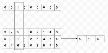
Another strategy is to use Hashing technique.
Generate K random permutations of 0.to.m-1 where ‘m’ is the number of grid ids. For each permutation, there will be one index where the value is 1 and all remaining indices are 0 (since its a one-hot encoding). The new value is the value of the permutation entry for the non-zero index.
Concatenate the numerical as well as the one-hot encoding vectors for each trip.
Where to store the feature representations ?
The features could be stored in a database for persistence. We can use NoSQL database such as Cassandra to store the feature values.
Feature table: (trip_id, feature_id, feature_name, value)
For real time inferencing we should also use some in-memory database such as Redis to store the feature values.
How to train the model using the features ?
We can train a Tensorflow Neural Network model which reads the training data from Hive and the features from Cassandra.
- Output layer consists of 7 nodes each with an sigmoid activation function.
- Loss function is categorical crossentropy.
- Train the network using Adam or Adagrad optimizer.
- For regularization use dropout in the hidden layers.
- For speeding up training use a BatchNorm layer after each hidden layer.
Following are the steps to train the model:
- Split the dataset into training, testing and validation (usually 80–20)
- Do the hyperparameter tuning (number of hidden layers, number if units in hidden layers, dropout etc.) using grid search cross validation (K-fold).
- The best hyperparameters are chosen based on the AUC score on validation dataset averaged over all the K runs.
- Final model is trained on the entire training data with the best hyperparameters.
How to evaluate the model offline ? Metrics ?
AUC Score
How to save the model and model weights, architecture etc. ?
Tensorflow models can be saved in multiple different ways.
- During training i.e. after each epoch we can save the model checkpoints using callbacks (so that even if we stop training we can start from wherever we have left). The model checkpoints consists of the model weights and index files. If the network is sharded, then weights corresponding to each shard are stored in separate files and the index file is like an hashmap from the weight (source layer, source node, dest layer, dest node) to the shard.
- After training, the model can be saved in SavedModel format which stores the model as Protobuf file.
- All of these checkpoints and protobuf files can be uploaded to S3 after training is completed.
<bucket_name>/<date>/<version>
How to train when the training data size is too huge for a single machine ?
There are multiple ways by which this can be achieved.
Generators
Instead of loading all training data in memory, use Python generators to generate the training data in batches and use Keras fit_generator method to train/validate Tensorflow model on these batches.
S3 Pipe Mode
Upload the training data in S3 instead of Hive and then use Pipe mode during training with Sagemaker. Data is directly streamed to the training algorithm instead of saving it on local disk and then loading in memory. Here we have network I/O which might slow down training.
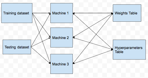
Distributed Training (Parameter Sharing)
- Split the training dataset across multiple nodes/machines.
- Copy the testing dataset in all the machines.
- Create a table in Cassandra to track the weights learned. (model_id, weights, loss, last_updated_timestamp)
- Create another table to track the cross validation runs. (model_id, machine_id, fold_num, hyperparameter_hash, hyperparameters, validation_loss)
- In each machine, divide the training set into K equal parts for K fold CV.
- Before running the hyperpaparmeter CV tuning job, update the hyperparameters table with the model_id, machine_id, fold_num, hyperparameters data. The hyperparameters is JSON string and is same for all fold_num coresponding to a model_id.
- After finding the validation loss for a hyperparameter setting update the validation_loss column corresponding to model_id, machine_id, fold_num and hyperparameters in Cassandra.
- To find the best hyperparameters for a model, do
SELECT hyperparameters
FROM
(SELECT model_id, hyperparameters, AVG(validation_loss) as loss GROUP BY model_id, hyperparameter_hash)
HAVING loss=MIN(loss)- Before each epoch, fetch the ‘weights’ from the weights table and run gradient descent on these set of weights.
- After finding the updated weights and the loss on the training data in one epoch, send the updated weights with the loss to Cassandra. If the timestamp is greater than the last_updated_timestamp then the weights and loss are overwritten in the weights table else they are ignored.
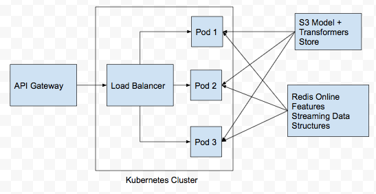
How to deploy the inferencing codes into production ?
- Instead of explicitly loading the Tensorflow SavedModel file and other index files for inferencing within Flask, we can use TF Serving to do that for us.
- But TF Serving do not handle feature preprocessing. For that we need Flask.
- Create Flask endpoints for inferencing.
- To make Flask multithreaded, use Gunicorn on top of Flask.
- Use Github+Jenkins to build a CI/CD Pipeline.
- Whenever a PR for the inferencing codes is created in Github, trigger Jenkins build i.e. run any unit and integration test cases and if all test cases passes, then build docker image and deploy the docker image in a Kubernetes cluster.
- Instead of a single docker container running both TF Serving and Flask+Gunicorn, create 2 separate docker containers so that they are decoupled.
- In Kubernetes, we would have 2 deployments and 2 services coresponding to the TF Serving and Flask/Gunicorn server.
- Use at-least 3 replicas for the pods running the docker services to allow for load balancing.
How to monitor the models in production ?
Setup logging and observability with Datadog or Cloudwatch (if using AWS).
Some performance metrics we can track are:
- Number of 5xx errors in the last 5 minutes.
- P99 latency every 5 minutes.
- Number of requests per second.
- CPU load across different nodes running the inferencing service.
- Memory usage across different nodes running the inferencing service.
- Number of Exceptions in the last 5 minutes.
Model metrics we should track:
- Data drift — For each feature pre-compute the mean and variance in the training dataset. In production compute the mean and variance of feature values in streaming way and after every 5 minutes, compute the KL Divergence between the training and production values.
How to do online evaluation ?
Using A/B Testing with “Number of sucessful bookings”.
We could have also used number of completed trips but it may happen that there was a cancellation after booking was made by either driver or rider which is not due to the surge_multipler shown since the rider has already accepted it and made the booking.
Another important metric is the number of pending booking requests every 5–10 minutes. Since our goal is to match the demand with the supply, this is an important metric. If the number of pending requests are high it implies that demand is more than supply.
For each booking attempt, if the booking is done we assign it a value of 1 else if rider does not make a booking we assign it a value of 0.
The base model (model0 or null hypothesis) in this case is that a rider is randomly shown a surge_multiplier i.e. each surge_multiplier has a probability of 1/7 of being shown to a rider.
Why not show surge_multiplier=1 to all riders ? Then it would be a biased model as everyone would book a ride and then it would lead to imbalance in the demand and supply of cabs as a result wait times will increase which will lead to rider frustation and uninstallations.
Our Tensorflow ML model is model1.
We perform chi-square test on the observations for 30 days. Divide the set of riders into 2 equal groups with one of them receiving surge_multipliers from model0 and another from model1.
Thus we would have 4 different counts:
- Number of users who booked after seeing surge_multiplier from model0
- Number of users who did not book after seeing surge_multiplier from model0
- Number of users who booked after seeing surge_multiplier from model1
- Number of users who did not book after seeing surge_multiplier from model1
We can compute chi-square score using the above 4 counts.
Pipeline
Training
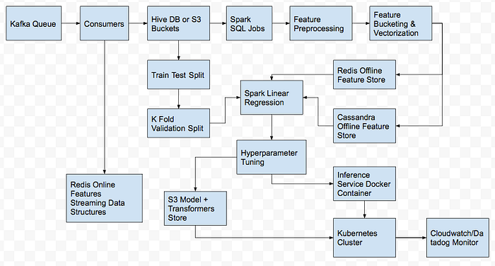
Inference