System Design — Google Maps

Abhijit Mondal

10 min readApr 11, 2022

Design the routing engine for Google Maps

Functional Requirements

Users must be able add new places to the map.
Users must be able to find the best route between two places on the map.

Non Functional Requirements

Availability — System should be highly available.
Scalability — System should scale when more new places are added to the map.
Durability — A place added should not get lost.
Low Latency — Searching and finding best routes should be as fast as possible.

Traffic and Throughput Requirements

Total number of users = 1 billion
Number of DAU = 200 million
Number of places = 100 million
Average number of new places added everyday = 10K
Number of routing queries per second = 10K
Average latency for routing queries = 100ms

The “On My Computer” Approach

How to encode the places on the map ?

Using Quad Tree.

class Coordinate {
    float latitude;
    float longitude;
}class QuadNode {
    Integer ID;
    QuadNode* NE;
    QuadNode* NW;
    QuadNode* SE;
    QuadNode* SW;
    Coordinate topLeft;
    Coordinate bottomRight;
    Boolean isLeafNode;
    List<Coordinate> coordinates;
}

To persist the data structure, we can store QuadNodes at each level of Quad Tree in each separate line of a text file. QuadNode object can be serialized as a JSON string. To identify a QuadNode object we can assign unique ID to each object.

{"ID":1,"NE":2,"NW":3,"SE":4,"SW":5,"topLeft":[20,30],"bottomRight":[50,60],"isLeafNode":'False',"coordinates":[[23,37],[35,43]]}
....

Only the leaf nodes contains the actual coordinates and each leaf node can contain upto a maximum of say 1000 coordinates.

How to find nearby places within X KMs from a given coordinate ?

If current node is a leaf node i.e. node.isLeafNode is True then for all node.coordinates check which are within X KMs from coordinate (euclidean distance) and add those to the final ‘result’ variable.
Else for each node.NW, node.NE, node.SW and node.SE, if the quadrant intersects with the circle centered at coordinate of radius X, then recursively call steps 1 & 2 on each quadrant.

How to find the shortest distance between 2 places on the Map ?

There are multiple possible approaches with various trade-offs on simplicity, correctness, speed at query time, speed at preprocessing time, memory for preprocessing etc.

Djikstra’s Algorithm:

Let dist[source][P] be the shortest distance between source and P. For a place Q, along the path from source to P, if there is a direct road from Q to P, then update:

dist[source][P] = dist[source][Q]+distance(Q, P) if dist[source][P] > dist[source][Q]+distance(Q, P) where distance(Q, P) is the distance from Q to P.

If the map and the road networks are relatively static, then we can cache the dist[source][P] for already computed source and destination pairs. If the source is same but destination changes many times, we can reuse the distances from the cache itself.
If dist[source][destination] is NULL in cache, then we compute source->P for all nodes P reachable from source and then cache them.

Also for all shortest paths from source to destination, if a place P lies along a shortest path then we can say that dist[P][dst] = dist[src][dst]-dist[src][P]. Thus we can also cache dist[P][dst] for all places P lying along the shortest paths from src to dst.

Pros:

Easy to understand and implement.
Good for short travel distances. If dest can be reached from source within 10KM, then we can explore roads and places that are only within 10KM (euclidean distance) from the source and destination.

For any given place P along src->dst, if dist[src][dst] <= 10KM
Then dist[src][P] + dist[P][dst] <= 10 for P to be a valid route.Implying dist[src][P] <= 10 and dist[P][dst] <= 10.
Since dist[x][y] >= Euclidean distance b/w x and y.Then we can filter only P's where Euclidean distance from src to P and P to dst <= 10KM.

Cons:

Time complexity is O((V+E)*logV). If the number of places and the number of roads (edges) are in millions, computing Djikstra if not already cached is very time consuming.
Everytime a place is added, all caches are invalidated because shortest path may be updated via the new place.
Not suitable for long distance travels.

Bi-Directional Djikstra:

Instead of adding paths only from source, we also add paths starting from the destination (but with reverse adjacency).

Whenever we find a common place P reachable from both source and destination, we do not explore further paths from P onwards. For all places P reachable from both src and dst:

dist[src][dst] = min(dist[src][P] + dist[dst][P]) over all P reachable from both src and dst

The advantage is that time taken is reduced by half from normal Djikstra.

A* Search:

In A*, we associate a cost with each path and explore paths with lower cost first.

Generally the cost of a path at a place P is:

cost = dist[src][P] + est_dist[P][dst]

where est_dist[P][dst] is the estimated distance from P to dst. Generally we take a lower bound on the distance such as Manhattan distance or Euclidean distance from P to dst.

In Djikstra, we do not consider the est_dist[P][dst] in the cost and the cost is only:

cost = dist[src][P]

If dst can be reached from P directly through Manhattan or Euclidean path, then A* is much faster as compared to Djikstra where we will still be exploring other possible paths which are not optimal.

Instead of using Manhattan or Euclidean distances as lower bound for the estimated distance from P to dst in the cost, we can use a much more stronger inequality i.e. Triangle Inequality.

Preselect N landmarks between src and dst. For a place P and landmark L, by triangle inequality:

dist[P][dst] + dist[dst][L] ≥ dist[P][L] where L is a landmark.
dist[P][dst] >= dist[P][L] - dist[dst][L]

For each landmark L, we precompute the shortest distances to all other places. Then for est_dist[P][dst] we take the smallest value of dist[P][L] — dist[dst][L] among all landmarks.

cost = dist[src][P] + min(dist[P][L] - dist[dst][L]) among all L.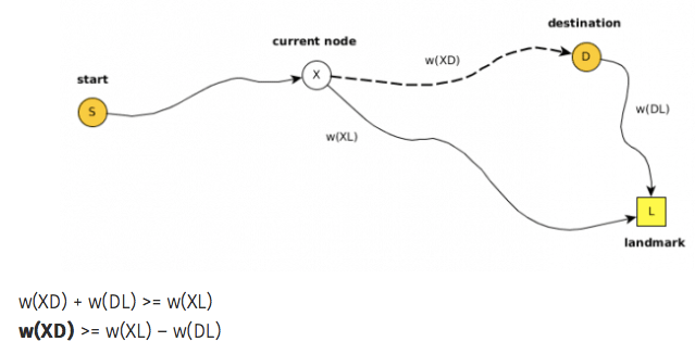

Pros and Cons are same as Djikstra.

Contraction Hierarchies:

The idea is to create shortcuts between pairs of places. For a path such as:

u — (3km) — v — (5km) — w

If the shortest path from u to w passes through v, then we can add a direct virtual edge from u to w with a weight of 8 km.

The idea is that in the first iteration, for each place u, do BFS to find the local neighborhood i.e. nearby places within K hops from ‘u’. Run Djikstra’s algorithm to find all shortest paths u — v — w, then add direct virtual edges u- — -w.

In the next iteration of contraction, running BFS+Djikstra’a algorithm will also take the virtual edges into account and thus will add virtual edges on top of virtual edges from previous iteration and so on.

At query time from the source, the longer virtual edges are given preference over shorter ones. Thus Djikstra’s algorithm will skip over many places (i.e. vertices) in the graph by following the virtual edges instead of the true edges.

Pros:

Many places and roads can be skipped during query time for shortest route.
Virtual edges can be computed periodically using background jobs i.e. we can run iteration k+1 anytime after iteration k without affecting the final results.
Shortest paths can be computed using Djikstra or A* algorithm.
Can work well for longer routes too.

Cons:

Requires preprocessing of road networks to compute virtual edges. Can be time consuming.
Requires additional memory to store virtual edges.

How to find the shortest path given the shortest distances from source to all other places ?

Maintain another table prev[u][v] which stores the previous place when the current place is v for the shortest path from u to v.

u — — — — — w-v

if dist[u][v] > dist[u][w]+dist[w][v] {
    dist[u][v] = dist[u][w]+dist[w][v]
    prev[u][v] = w
}

Then we can unfold prev[src][dst] to get the shortest path.

curr = dst
path = []while curr is not NULL {
    path = [curr] + path
    curr = prev[src][curr]
}

What are the drawbacks of the “single machine” approach ?

Estimated number of places for 5 years = 100 million + 10000*365*5 = 119 million.

Number of bits required to store unique ID for each place = log2(119 million) = 27 bits

Size of the dist[][] in-memory table for every pair of places = 119million*119million*64bits (for distance)=100PB.

Size of the prev[][] in-memory table for every pair of places = 119million*119million*27bits (for place id)=43PB.

Since it is infeasible to store distances for every pair of places and also every pair do not make sense when one place is one continent and another in another continent. We can make use of LRU cache which stores dist and prev for the most recently used 100 billion src, dst pairs.

Thus size of dist[][] in LRU cache = 100billion*64 bits = 745GB.

Size of prev[][] in LRU cache = 100billion*27 bits = 314GB.

Assuming an average serving latency of 100ms for each routing query, number of requests that can be served (for 8 core CPU)= 8*1000/100 = 80. But we need to serve 10K requests per second from routing engine.

Using Distributed Systems

How many nodes are required for the routing engine ?

Assuming each machine holds around 64GB RAM, total number of machines required for caching = (745+314)GB/64GB = 17.

But from the perspective of the requests per second, we need 10000/80 = 125 machines because each machine can support about 80 requests per second but our requirement is for 10K.

How to partition the distance/prev table ?

Possible strategies are:

Based on the source — For a given src, prev[src][] is stored in a single partition. But since for the shortest path queries, we need to query prev[][] with different src everytime, this does not help us much as anyways we need to query from multiple partitions.
Random — Randomly select (src, dst) pairs and assign them to a partition: Hash(src||dst)%N. No hot partition issues but again we need to query multiple partitions to find the best path.
Based on City— For a given city, prev[src][] for all src in the city are stored in a single partition. This could lead to uneven distribution as some cities would have many places whereas some very few.
Based on Quad Tree Grids — For a given grid id, prev[src][] for all src in the grid id i.e. list of coordinates under that QuadNode are stored in a single partition. Same problem here since grids are non-uniform. Better alternative is to use R-Trees instead of Quad Trees.

How writes are routed based on partitioning ?

We can maintain a Metadata service to map quad tree leaf node grid ids to machine ids. Create a HashMap of quad tree grid id to machine id:

HashMap A: QuadNode.ID -> (host, ip)

When a new place is added, the coordinate is first converted into QuadNode.ID, select a host based on number of active assignments (roughly equal) in a round robin fashion and then map the grid ID to the host and ip.

Similarly for queries, convert the coordinate to quad tree leaf node ID, then lookup the HashMap from the Metadata service to go the host having data for a given src. Observe that it is particularly useful to have all nearby places in the same machine (host) else everytime we have to query the Metadata service to shuffle between machines.

But for very long routes, we may need to lookup Meatadata service multiple times. In order to check whether prev[src][] is in the same machine or not without looking up the Metadata service, we can use Bloom Filters within each machine to do fast lookup if prev[src][] can be found in the same machine or not.

What happens when a grid gets split ?

When a grid is split, it is divided into 4 parts each having an unique ID. Thus we need to re-map all the coordinates in the original grid ID to the new grid IDs. Although it is not guaranteed that splitting one grid will produce 4 new leaf nodes since depending on the constraints set for the maximum number of coordinates under one leaf, it can further subdivide into 4 grids. Thus the final number of re-mappings would be 4+3k i.e. 4, 7, 10 etc.

One possible strategy to avoid constant re-mappings would be to consider higher level grid ids instead of leaf nodes.

How to achieve high availability ?

Given that the routing engine is using an in-memory table (2D matrix) for caching the distances and prev, if we only have a single instance of dist[][] or prev[][] in the event of crash, this data would be lost.

We can replicate the data across multiple machines for fault tolerance.

At-least 3 replicas for each dist[][] and prev[][] matrices.

What is the replication strategy ?

Two important things to consider here are:

Reads should be fast.
Writes should be durable.

We can use Master-Slave replication.
We would have a single master instance and multiple read replicas. All writes happen at the master which is then replicated to all read replicas. All reads happen from read replicas through a load balancer.

Replication can be synchronous, asynchronous or semi-synchronous.

With synchronous replication writes will be slower as response to client has to wait for all ACKs from the read replicas but reads are strongly consistent. Whereas with fully asynchronous, writes are fast as client do not wait for ACKs from read replicas but reads are eventually consistent i.e. reads immediately after writes may not see the newly added places.

With semi-synchronous replication clients wait for ACKs from at-least K read replicas where K < number of read replicas. The probability of not seeing the newly added place is reduced but writes become slower as compared to fully asynchronous.

System Design — Google Maps

Similar Questions

Functional Requirements

Non Functional Requirements

Traffic and Throughput Requirements

The “On My Computer” Approach

Using Distributed Systems

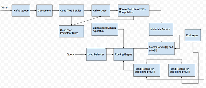
The Pipeline

Resources

Written by Abhijit Mondal